Mastering the IF AND Formula in Excel: A Beginner's Guide to Data Analysis- Video Tutorial

 Welcome to our video tutorial on how to use the IF and AND formula in Excel to determine whether students have passed or failed based on attendance and marks. In this tutorial, we will be walking you through each step of the process, from creating a new column in your Excel sheet to applying the formula to the rest of the students. We will also be discussing the importance of data analysis and decision making in today's world, and how mastering the IF and AND formula can help you make better decisions with your data. So, whether you're a student, a teacher, or a professional, this tutorial will provide you with the knowledge and skills you need to analyze your data and make data-driven decisions. So, grab your computer, and let's get started!

Mastering the IF Formula: A Guide to Calculating Incentives in Excel

 In the world of sales, incentives can be a powerful motivator for employees to reach their targets and exceed them. One way to calculate these incentives is by using the IF formula in Excel.

The IF formula is a logical function in Excel that allows you to test a condition and then return a value based on the outcome of that test. In the context of incentive calculation, this can be used to determine the amount of incentive an employee should receive based on their sales performance.

To use the IF formula for incentive calculation, you'll first need to set up a spreadsheet with the following columns: employee name, sales and incentive. Next, you'll need to determine the criteria for calculating the incentive. This could be based on a percentage of sales or a fixed amount for reaching or exceeding the sales target.

Once you have the criteria in place, you can use the IF formula to test whether an employee's actual sales meet or exceed the target and calculate the incentive accordingly. For example, if the sales target is Rs.50000 and the incentive is 5% of sales for reaching or exceeding the target, the formula would be:

=IF(B2>=A2,B2*5%, "")

We can see step by step procedure with images

1.Organize the data in tabular form with columns as Employee name, Sales and Incentive

2.Start typing if formula with logical test as shown in image.

3.If logical test is true then 5% of incentive to be calculated. Hence type as per below image.

4.If logical test is false, then 1% incentive to be calculated as shown below.

5.Now press enter key and drag down the formula up to last cell.

6.You can see the incentive calculated for all employees. For better visualization we will format the numbers into currency.

In this way if formula is used for incentive calculation.

👉Click here for watching video tutorial to calculate incentive

The IF Formula for Incentive Calculations: A Step-by-Step video Tutorial

 

Video tutorial- Pass or Fail: Using the IF Formula to Calculate Student Results in Excel

Please watch a video to learn if formula
 

Pass or Fail: Using the IF Formula to Calculate Student Results in Excel

In Excel, you can use the IF formula to calculate whether a student has passed or failed based on their marks. The basic syntax for the formula is:

=IF(condition, value if true, value if false)

To check if a student's marks are greater than or equal to 40, the condition would be:

A1 >= 40 (A1 is the cell where student's marks are stored)

If the condition is true (i.e. the student's marks are greater than or equal to 40), the formula would return "Pass". If the condition is false (i.e. the student's marks are less than 40), the formula would return "Fail". So the formula would be:

=IF(A1 >= 40, "Pass", "Fail")

You can also use this formula in other cells to check for other students.

Below is the step wise procedure shown with images for better understanding.

To watch a video tutorial you can visit the link👉Video Tutorial

 Otherwise you can learn through stepwise procedure written below

1. Write all the data in organized way as shown in below picture

2. We have decided the criteria of marks. So we will enter a formula accordingly. Type a criteria as logical test.

3. Now type a result to be printed if criteria is met. i.e. if marks are >=40, then Pass should be printed.

4.Now type a result to be printed if marks are less than 40 i.e. Fail

5. Now press Enter key and drag the formula up to last cell.

6.In this way result of all student is calculated in few seconds using if formula. In below image failed students are highlighted with Red color

👉Click here to learn more about if formula

How to calculate grades of students using Excel | एक्सेल वापरून विद्यार्थ्यांच्या ग्रेडची गणना कशी करायची

 We can calculate grades by using If formula.

What is if formula?

"If" सूत्र म्हणजे काय?

The IF function in Excel is used to perform a logical test and return one value if the test is true and another value if the test is false. The basic syntax of the IF function is as follows:

=IF(logical_test, value_if_true, value_if_false)

The "logical_test" is a comparison or logical statement that returns either TRUE or FALSE. The "value_if_true" is the value that is returned if the logical test is true. The "value_if_false" is the value that is returned if the logical test is false.

For example, if you wanted to test if a cell in a spreadsheet contains a value greater than 100 and return "Greater than 100" if true and "Less than or equal to 100" if false, you would use the following formula:

=IF(A1>100, "Greater than 100", "Less than or equal to 100")

where A1 is the cell containing the value to be tested.

Excel मधील IF फंक्शन तार्किक चाचणी करण्यासाठी आणि चाचणी सत्य असल्यास एक मूल्य आणि चाचणी खोटी असल्यास दुसरे मूल्य परत करण्यासाठी वापरली जाते. IF फंक्शनची मूलभूत वाक्यरचना खालीलप्रमाणे आहे:

=IF(लॉजिकल_टेस्ट, value_if_true, value_if_false)

"लॉजिकल_टेस्ट" हे एक तुलना किंवा तार्किक विधान आहे जे सत्य किंवा असत्य मिळवते. "value_if_true" हे मूल्य आहे जे तार्किक चाचणी सत्य असल्यास परत केले जाते. "value_if_false" हे मूल्य आहे जे तार्किक चाचणी चुकीचे असल्यास परत केले जाते.

उदाहरणार्थ, जर तुम्हाला स्प्रेडशीटमधील सेलमध्ये १०० पेक्षा जास्त मूल्य आहे की नाही हे तपासायचे असेल आणि खरे असल्यास "100 पेक्षा मोठे" आणि असत्य असल्यास "100 पेक्षा कमी किंवा बरोबरीचे" परत करा, तर तुम्ही खालील सूत्र वापराल:

=IF(A1>100, "100 पेक्षा जास्त", "100 पेक्षा कमी किंवा समान")

जेथे A1 हा सेल आहे ज्यामध्ये चाचणी करायची आहे.

Today let us see how ifs formula works.

(Click here to learn If formula with example)

Today we will learn how to use ifs formula to analyze the result of students. We have marks of seven students and we want to show the result of students in Grade column by using multiple conditions.

 आज आपण विद्यार्थ्यांच्या निकालाचे विश्लेषण करण्यासाठी ifs फॉर्म्युला कसा वापरायचा ते शिकू. आमच्याकडे सात विद्यार्थ्यांचे गुण आहेत आणि आम्हाला खालील अटी वापरून ग्रेड कॉलममध्ये विद्यार्थ्यांचा निकाल दाखवायचा आहे.

Please follow below steps to analyze results using if formula

इफ फॉर्म्युला वापरून निकालांचे विश्लेषण करण्यासाठी कृपया खालील चरणांचे अनुसरण करा

Step 1. Start typing ifs formula in 1^st cell of Grade column as =ifs and type 1^st condition as shown in below table and press comma(,). Once you press comma you can start writing second condition.

ग्रेड कॉलमच्या 1ल्या सेलमध्ये ifs फॉर्म्युला =ifs म्हणून टाइप करणे सुरू करा आणि खालील टेबलमध्ये दाखवल्याप्रमाणे 1ली कंडिशन टाइप करा आणि स्वल्पविराम(,) दाबा. एकदा तुम्ही स्वल्पविराम दाबल्यानंतर तुम्ही दुसरी अट लिहायला सुरुवात करू शकता.

Step 2.Type second condition in a formula as shown in below table. After completion of 2^nd condition press comma(,).

खालील सारणीमध्ये दर्शविल्याप्रमाणे सूत्रामध्ये दुसरी स्थिती टाइप करा. दुसरी अट पूर्ण झाल्यानंतर स्वल्पविराम(,) दाबा.

Step 3. Once you enter comma(,), you can start writing 3^rd condition. So start writing condition as shown in below table

एकदा तुम्ही स्वल्पविराम(,) एंटर केल्यावर तुम्ही 3री अट लिहायला सुरुवात करू शकता. तर खालील तक्त्यामध्ये दर्शविल्याप्रमाणे अटी लिहिण्यास सुरुवात करा

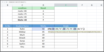
Step 4. This step is crucial step in this formula. We know that Below 40, grade should be F. So to mention that this is the last  condition, type ‘True’ as shown in below table.

ही पायरी या सूत्रातील महत्त्वाची पायरी आहे. तुम्हाला माहीत आहे की 40 च्या खाली, ग्रेड F असावा. त्यामुळे ही शेवटची अट आहे हे नमूद करण्यासाठी, खालील तक्त्यामध्ये दाखवल्याप्रमाणे 'True' टाइप करा.

Step 5. Once you type ‘True’, you will write a final condition. This condition will mean that if all 1^st three conditions are not true then “F” will be printed. Type the condition and press Enter. Please refer below table.

एकदा तुम्ही 'True' टाइप केल्यावर तुम्ही अंतिम अट लिहाल. या स्थितीचा अर्थ असा होईल की जर सर्व 1ल्या तीन अटी सत्य नसतील तर "F" छापले जाईल. कंडिशन टाइप करा आणि एंटर दाबा. कृपया खालील सारणी पहा.

Step 6. Do the selection from 1^st cell in Grade column to last cell in Grade column and press Ctrl+D. We will get the result of each student.

ग्रेड कॉलममधील पहिल्या सेलपासून ग्रेड कॉलममधील शेवटच्या सेलपर्यंत निवड करा आणि Ctrl+D दाबा. प्रत्येक विद्यार्थ्याचा निकाल मिळेल.

In this way even if you have 100 or more than 100 students data, you can calculate their grades in few minutes.

अशा प्रकारे तुमच्याकडे 100 किंवा 100 पेक्षा जास्त विद्यार्थ्यांचा डेटा असला तरीही, तुम्ही काही मिनिटांत त्यांच्या ग्रेडची गणना करू शकता.

We can use the same if formula for deciding the result as Pass or Fail.

Top 30 Most Useful Excel Shortcut keys

Excel shortcut keys are important because they can save a significant amount of time and effort when working with large or complex spreadsheets. With shortcut keys, you can perform common tasks, such as copying and pasting, with just a few keystrokes, rather than having to navigate through menus and ribbons to find the appropriate command. Additionally, shortcut keys can help you work more efficiently by allowing you to quickly access frequently used commands and tools.

Shortcut keys can also help reduce the risk of errors, as they allow you to perform tasks quickly and accurately, without having to take your hands off the keyboard. This can be particularly useful when working with large amounts of data, as it allows you to quickly navigate through your spreadsheet and make changes without having to constantly move your cursor around the screen.

Here are some important shortcut keys you should know:👇

1	Ctrl + C	Copy
2	Ctrl + V	Paste
3	Ctrl + X	Cut
4	Ctrl + Z	Undo
5	Ctrl + Y	Redo
6	Ctrl + A	Select all
7	Ctrl + F	Find and Replace
8	Ctrl + P	Print
9	Ctrl + S	Save
10	Ctrl + N	New workbook
11	Ctrl + O	Open workbook
12	Ctrl + W	Close workbook
13	Ctrl + Tab	Switch between open workbooks
14	Ctrl + Shift + Tab	Switch to previous workbook
15	Ctrl + Page Up	Switch to previous worksheet
16	Ctrl + Page Down	Switch to next worksheet
17	Ctrl + Home	Go to the beginning of a worksheet
18	Ctrl + End	Go to the end of a worksheet
19	Ctrl + Arrow keys	Move to the edge of a data range
20	Shift + Arrow keys	Select a range of cells
21	Ctrl + Shift + Arrow keys	Select a range of cells and all cells in between
22	F2	Edit cell
23	F5	Go to a specific cell or range
24	F7	Spell check
25	F11	Create a chart
26	Alt + =	Auto-sum
27	Ctrl + Shift + &	Apply border to selected cells
28	Ctrl + Shift + _	Remove cell borders
29	Ctrl + Shift + +	Insert a new row or column
30	Ctrl + -	Delete selected row or column

In this way, using shortcut keys can help to improve your productivity as you don't have to spend time looking for the command you need, this can add up over time, especially when working on large projects or with large amounts of data. So, mastering Excel shortcut keys can make you a more efficient and effective user of the software.