Best hospitals in chandwad

If you are a student living in a hostel or if you are new in chandwad , here is the list of best hospitals in Chandwad,Tal.Chandwad Dis.Nashik

1.Dwarkadhish Hospital

This hospital is situated at distance of 200m from Chandwad bus stand. This is one of the renouned hospital in Chandwad. 

2.Modi Hospital

This hospital in situated exactly near the bus stand of Chandwad. This is one of the oldest hospitals in Chandwad.

3.Mahale Hospital

This hospital is located in Davkhar Nagar of Chandwad.  This hospital has the best facilities amongst all hospitals in Chandwad. Though it is in remote area from main city, it has maximum patients due to best results getting from treatment.

4.P.K.Pawar memorial hospital

In case if any severe accidental damage , you can visit this hospital in Chandwad. This hospital is located exactly near the Chandwad market.

5.Sushrut Hospital

This is also one of the oldest hospitals in Chandwad. It is located in main city of Chandwad.

दुःख अडवायला उंबऱ्यासारखा। Dukh advayla umbaryasarkha

मैत्री वरील कविता

दुःख अडवायला उंबऱ्यासारखा ,

मित्र वनव्यामध्ये गारव्यासारखा……… १

वाट चुकणार नाही जीवनभर कोणी,

एक तू मित्र कर आरशासारखा,

मित्र वनव्यामध्ये गारव्यासारखा……. २

आत्महत्याच करणार नाही कोणी,

मित्र असला जवळ जर मनासारखा,

मित्र वनव्यामध्ये गारव्यासारखा…….. ३

त्रासलो जिंदगी चाळताना पुन्हा,

बस धडा मैत्री वाचण्यासारखा,

मित्र वनव्यामध्ये गारव्यासारखा……. ४

मैत्री चाटते गाय होऊन मना,

जा बिलग तू तिला वासरासारखा,

मित्र वनव्यामध्ये गारव्यासारखा…… ५

कवी अनंत राऊत

MS Excel: How to use countif function

Purpose of using Countif formula

Countif formula is used to count the number of cells that meet specific single criteria

 

What is the output of countif formula?

This formula returns the count of cells  in the selected range which satisfy the mentioned criteria

 

What are the steps to use countif formula?

1. Select a cell where you want the output

2. Type a formula like this =countif

3. Double click on Countif formula

4. Now it will ask range so select the range of cells. This range contains the criteria which we are going to apply

5. Press comma(,)

6. Enter a criteria. If it is a text then type it in double inverted comma “criteria”. If criteria is in a numeric form then no need to press “”.

7. Then hit enter

We will see the example

Suppose we have a list of students and their result (Pass/Fail) and we want to count the number of Pass students and number of Fail students then we will use countif function

Now select a cell and type =countif formula and double click on it. Now select a range as show in picture and press comma ,

We want to count Pass students. Hence type “Pass” in criteria argument.

Now hit enter to see the result as count of pass students

Similarly countif can be used to count Fail students. Follow the same steps up to the selection of range and type Fail in criteria.

Hit enter key. You can see the count of Fail students

In this way countif function has its application from basic level to advance level. This can improve you efficiency of working on excel.

Click here to learn if formula

SUMIF formula: How to use it

Basically sum if formula is used to sum the values based on criteria specified by you.

Syntax of SUMIF formula are explained below

SUMIF(range, criteria, [sum_range])

"Range" is the range of cells you want to evaluate.

"Criteria" is the condition or criteria that you want to apply.

"Sum_range" is the range of cells to sum if the criteria or condition is met.

Let us see how to use it practically with example. 

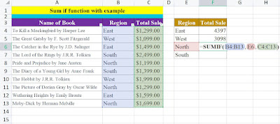
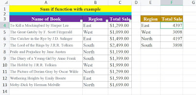
So, if you have sold different books in different regions and you have its data maintained in sheet. Then you can use sumif formula to calculate region wise total sale of all books.

Steps to do that are as below.

Step 1. Write a data in organized form

Step 2. Start writing sumif formula as "=sumif"

Step 3. Now formula will ask range to select. So select the range from which criteria will be selected.

Then press comma(,) and select the criteria. Here our criteria is East region. Hence select East and press comma(,).

Step 4. Now formula will ask to select sum range. Select the cells from which want to sum the values.

Step 5. Now press the Enter key and you will be able to see the total sale in East region

Step 6. Follow the step 1 to 5 for remaining regions. You will get Total sale of all regions.

As shown in above pictures, you will get the required result as per applied formula. This is the way to use SUMIF formula. It can be used for various types of data analysis in you professional or personal life. SUMIF formula can also be used in project management, inventory analysis, sales analysis, financial analysis.

Excel Tips & Tricks: How to Use the "IFERROR" Formula

Excel is a powerful tool for organizing, analyzing and presenting data. However, even the most experienced users can make mistakes. One of the most common problems in Excel is the appearance of error messages, such as #N/A, #VALUE, #REF, and others. Fortunately, the "if error" formula in Excel can help you avoid these errors and ensure your data is accurate.

In this blog, we’ll explore what the "if error" formula is, how to use it.

What is the "if error" formula in Excel?

The "if error" formula in Excel is a conditional formula that returns a specific value if a formula generates an error. It allows you to control the error messages that appear in your data and replaces them with a value or text of your choice. The formula is written as follows:

=IFERROR(value, [value_if_error])

The "value" argument is the formula or expression you want to evaluate. The "[value_if_error]" argument is the value or text you want to appear if an error occurs.

How to Use the "if error" Formula in Excel?

Using the "if error" formula in Excel is easy. Simply follow these steps:

1.Enter the formula or expression you want to evaluate in a cell.

2.Select the cell where you want to apply the "if error" formula.

3.Enter the formula =IFERROR(value, [value_if_error]) in the formula bar.

4.Replace "value" with the cell reference containing the formula or expression you want to evaluate.

5.Replace "[value_if_error]" with the value or text you want to appear if an error occurs.

Press the Enter key to apply the formula.

Do watch a video to understand this IF ERROR formula 👇

The "IFERROR" formula in Excel can be used with many other functions such as:

1.VLOOKUP

2.INDEX/MATCH

3.SUMIF/SUMIFS

4.AVERAGEIF/AVERAGEIFS

5.COUNTIF/COUNTIFS

6.DIVIDE (to avoid "#DIV/0!" errors)

7.Nested IF statements

It can also be used with text and date functions like LEFT, RIGHT, CONCATENATE, and DATE.

Excel Mastery: Mastering the IF-OR Function for Player Selection in Sports Data Analysis

Excel is a powerful tool that allows you to organize, analyze, and visualize data in various ways. One of the most fundamental functions in Excel is the IF-OR function, which is used to test multiple conditions and return a specific result based on those conditions. In this blog post, we will explore how to use the IF-OR function in Excel using a tabular data set of player scores to determine player selection.

The IF-OR function in Excel is written as "=IF(OR(condition1, condition2, ...), value_if_true, value_if_false)". The function will test the conditions specified in the parentheses and return the value specified in "value_if_true" if any of the conditions are true, or the value specified in "value_if_false" if all of the conditions are false.

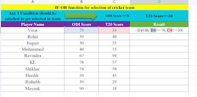
For our example, we will use the tabular data of player names, ODI scores, and T20 scores, and we want to add a column that will show whether the player is "Selected" or "Not Selected" based on their scores. The criteria for selection is that a player's ODI score must be at least 70, or their T20 score must be at least 30.

Step1. Write a data in tabular form as shown in below picture

Step2. With respect to predefined conditions start typing formula as shown in below picture

Step3.Type the values as per selection criteria

Step4.Press enter key and drag it up to last cell

As we can see, the IF-OR function has allowed us to quickly and easily test multiple conditions and return a specific result based on those conditions. This is just one of the many ways that the IF-OR function can be used in Excel, and understanding how to use it can be a valuable tool in organizing and analyzing data.

It's important to note that in this case we used OR function instead of AND to check both the conditions, as we want player to be selected if either of the score meet the criteria.

Click here to learn more about if formula

Click here to learn how to calculate incentive using IF formula

Mastering the IF AND Formula in Excel: A Beginner's Guide to Data Analysis

Welcome to our latest blog post on the power of the IF AND formula in Excel. Whether you're a student, a business professional, or just someone who wants to organize and analyze data, Excel is an incredibly useful tool to have in your arsenal. One of the most powerful features in Excel is the ability to use logical formulas, such as IF and AND, to make sense of your data and make informed decisions. In this blog post, we will be diving deep into the IF AND formula, explaining what it is, how it works, and providing examples of how you can use it in your own data analysis. 

We will also be providing examples of how the IF AND formula can be used in real-world scenarios, such as determining the passing or failing of students based on attendance and marks. So, whether you're a beginner or an advanced Excel user, keep reading to learn more about the IF AND formula and how it can help you make sense of your data.

Let's learn the IF AND function to decide the result of students as Pass or Fail.

Criteria to pass the exam- Attendance>=75% and Marks>=50

To determine whether each student has passed or failed based on attendance and marks using the IF and AND formula, you can use the following formula in Excel:

=IF(AND(B4>75,C4>50),"Pass","Fail")

(Click here to watch video tutorial)

In this formula, B4 and C4 represent the Attendance(%) and Marks respectively for the first student (ohn Smith). You can then drag the formula down to the rest of the cells in the "Pass/Fail" column to apply it to the rest of the students.

Step 1: Create a new column in your Excel sheet called "Result" where you want to show the results.

Step 2: Select the first cell in the "Result"  column. In this example, it will be D4.

Step 3: Type the following formula in the selected cell: =IF(AND(B4>75,C4>50),"Pass","Fail")

Step 4: Press Enter to apply the formula to the selected cell.

Step 5: Drag the fill handle (the small square located in the bottom-right corner of the selected cell) down to the rest of the cells in the "Result"  column to apply the formula to the rest of the students.

Step 6: Observe the results in the "Result"  column. If the student has attendance more than 75% and marks more than 50, the cell will show "Pass" otherwise "Fail".

In conclusion, the IF and AND formula in Excel is a powerful tool for data analysis that allows you to make decisions based on multiple conditions. By using this formula, you can quickly and easily determine whether students have passed or failed based on attendance and marks. This guide provides a step-by-step tutorial on how to use the IF and AND formula in Excel and this formula can be used in many other scenarios where multiple conditions are to be evaluated.

By mastering the IF and AND formula, you can improve your data analysis skills and make better decisions with your data.